Ray Tracers

The calculation of seismic travel times is a cornerstone for the migration and stacking approach. Qseek supports different ray tracers for travel time calculation, which can be adapted for different geological settings.

Constant Velocity

The constant velocity models is trivial and follows:

\[ t_{P} = \frac{d}{v_P} \]

This module is used for simple use cases and cross-referencing testing.

ConstantVelocityTracer Module

Travel time tracer with a constant velocity.

Config ConstantVelocityTracerJSON

phase: constant:P: Name of the phase.
velocity: 5000.0: Constant velocity of the phase in m/s.

JSON for ConstantVelocityTracer

{
  "tracer": "ConstantVelocityTracer",
  "phase": "constant:P",
  "velocity": 5000.0
}

1D Layered Model

Calculation of travel times in 1D layered media is based on the Pyrocko Cake ray tracer.

Pyrocko Cake Ray Tracer Pyrocko Cake 1D ray tracer for travel time calculation in 1D layered media

CakeTracer Module

Travel time ray tracer for 1D layered earth models.

Config CakeTracerJSON

phases: Dictionary of phases and timings to calculate.
earthmodel: Earth model to calculate travel times for.
trim_earth_model_depth: True: Trim earth model to max depth of the octree.
lut_cache_size: Size of the LUT cache. Default is 2G.

JSON for CakeTracer

{
  "tracer": "CakeTracer",
  "phases": {
    "cake:P": {
      "definition": "P,p"
    },
    "cake:S": {
      "definition": "S,s"
    }
  },
  "earthmodel": {
    "filename": "/home/marius/.cache/qseek/velocity_models/default.nd",
    "format": "nd",
    "crust2_profile": ""
  },
  "trim_earth_model_depth": true,
  "lut_cache_size": 2147483648
}

3D Fast Marching

We implement the fast marching method for calculating first arrivals of waves in 3D volumes. Currently three different 3D velocity models are supported:

Import NonLinLoc 3D velocity model
1D layered model 🥞
Constant velocity, mainly for testing purposes 🥼

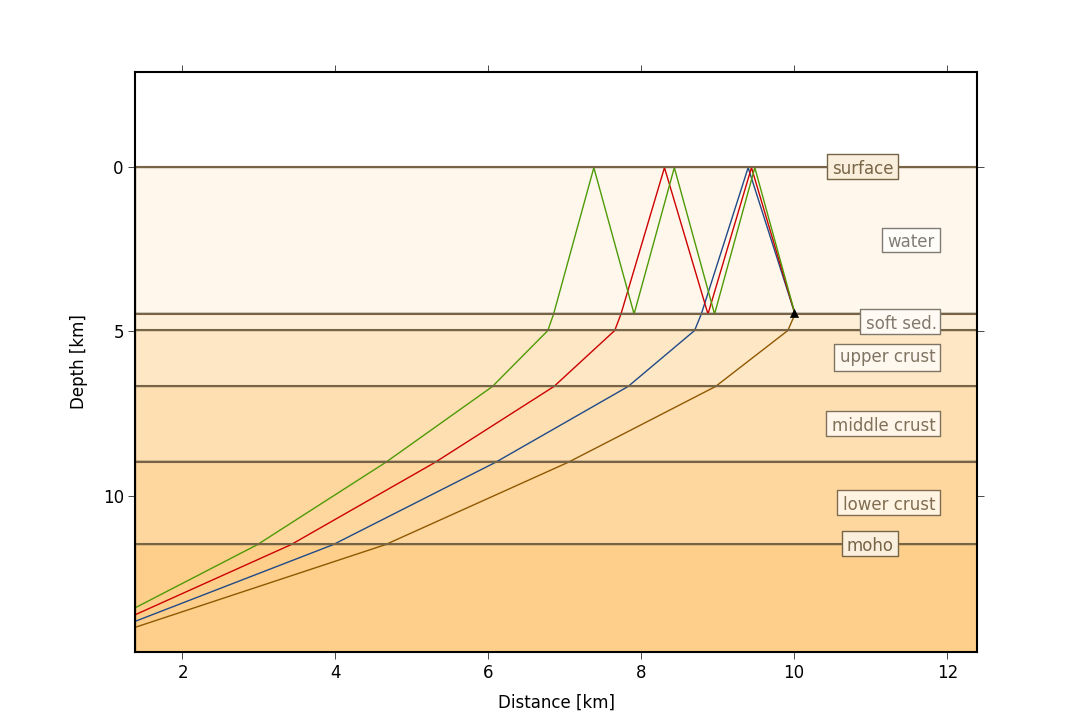
Fast Marhing Concept Conceptual 2D visualisation for seismic traveltimes calculation in heterogenous media using the fast-marching method for the Eikonal solution is presented. Traveltimes from the receiving station at the surface (indicated by a yellow triangle) towards the subsurface grid are calculated, resulting in station-specifig traveltimes for all potential source locations simultaneously.

FastMarchingTracer Module

Travel time ray tracer using the Fast Marching Method for 3D earth models.

Config FastMarchingTracerJSON

interpolation_method: nearest | linear | cubic: Interpolation method for travel times in the volume. Choose from nearest, linear or cubic.
nthreads: 0: Number of threads to use for travel time. If set to 0, cpu_count*2 will be used.
lut_cache_size: Size of the LUT cache. Default is 2G.
velocity_model: Velocity model for the ray tracer.
implementation: pyrocko | scikit-fmm: Implementation of the Fast Marching Method. Pyrocko only supports first-order FMM for now.

JSON for FastMarchingTracer

{
  "tracer": "FastMarchingRayTracer",
  "phase": "fm:P",
  "interpolation_method": "cubic",
  "nthreads": 0,
  "lut_cache_size": 2147483648,
  "velocity_model": {
    "model": "Constant3DVelocityModel",
    "grid_spacing": "octree",
    "velocity": 5000.0
  },
  "implementation": "scikit-fmm"
}

Visualizing 3D Models

For quality check, all 3D velocity models are exported to vtk/ folder as .vti files. Use ParaView to inspect and explore the velocity models.

Velocity model FORGE Seismic velocity model of the Utah FORGE testbed site, visualized in ParaView.